Reference paper. More detailed descriptions of the FLUXNET2015 dataset and the ONEFlux processing pipeline are available in the dataset reference paper, co-authored by data teams and members of all site teams contributing to FLUXNET2015 Tier One sites:
Pastorello, G., Trotta, C., Canfora, E. et al. The FLUXNET2015 dataset and the ONEFlux processing pipeline for eddy covariance data. Sci Data 7, 225 (2020). https://doi.org/10.1038/s41597-020-0534-3
[.bib, .ris]
The data processing pipeline for the FLUXNET2015 Dataset was developed in a collaboration between personnel from the European Ecosystem Fluxes Database, ICOS Ecosystem Thematic Centre (ICOS-ETC) and the AmeriFlux Management Project (AMP). It adapts code developed by the community, integrating with code developed by the teams into a consistent and uniform data processing pipeline. The starting point for the data processing is half-hourly data collected and processed at FLUXNET sites. The pipeline generates uniform and high quality derived data products suitable for studies requiring intercomparability of data from multiple sites. The harmonization and data quality control activities are particularly important for the FLUXNET2015 Dataset. Regional network coordination offices, in particular for OzFLUX-TERN, ChinaFlux, AsiaFlux, and FLUXNET-Canada are participating in the harmonization and data quality screening for the sites in their networks.
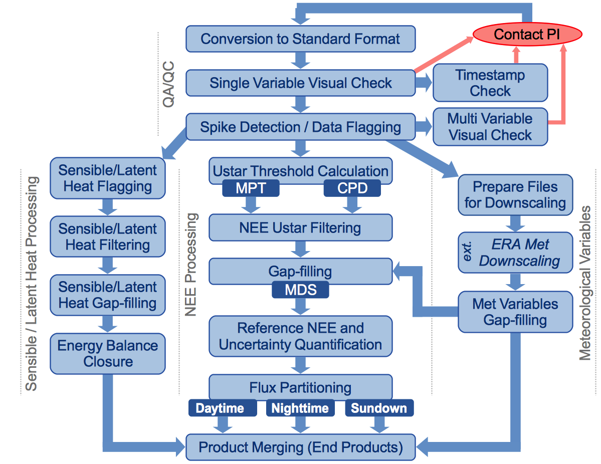 Figure 1. Processing Pipeline for FLUXNET2015 Release.
Temporal aggregations are generated at last step using each variable. These are all concatenated into the data distribution formats at the Product Merging step, which generates the final file representation for data products at all temporal aggregation resolutions.
1. QA/QC Procedures
Before product generation starts, data for each site goes through quality assurance / quality control (QA/QC) steps tailored to the generation of these derived data products (e.g., gap-filling or uncertainty estimation). A few of these QA/QC steps are described in PASTORELLO et al. 2014 (eScience). Quality checks are done over single variables (e.g., overall trends at multiple temporal resolutions), multiple/combined variables (e.g., variables that should vary comparably), or can be more specialized tests (e.g., comparing measured radiation to the maximum, top of the atmosphere radiation expected for a given location).
2. Micrometeorological Processing
Meteorological data includes at the moment a selection of variables that will be expanded in the next incremental releases. The variables are gapfilled with MDS but, for a selection of them where it was possible, also downscaled at site level from ERA-interim reanalysis data following the method described by Vuichard and Papale 2015 (ESSD). A proposed optimal combination of the two products is also produced (identified with _F).
Half hourly or hourly:
The file contain a set of meteorological variables gapfilled and/or downscaled from the ERA-interim dataset. The downscaling both in space (from cell to tower) and time (6 hourly to half hourly) is applied to seven variables using regressions with the site measurements when available according to the method described in Vuichard and Papale 2015.
The gapfilling of the site level measurements have been done using the MDS method as described in Reichstein et al. 2005.
For the variables where the ERA-interim downscaling has been applied, a merged version using the MDS gapfilled and the downscaled is also provided.
Daily:
The file contain a set of meteorological variables gapfilled and/or downscaled from the ERA-interim dataset aggregated at daily time resolution. The downscaling both in space (from cell to tower) and time (6 hourly to half hourly) is applied to seven variables using regressions with the site measurements when available according to the method described in Vuichard and Papale 2015.
The gapfilling of the site level measurements have been done using the MDS method as described in Reichstein et al. 2005.
For the variables where the ERA-interim downscaling has been applied, a merged version using the MDS gapfilled and the downscaled is also provided.
Weekly:
The file contain a set of meteorological variables gapfilled and/or downscaled from the ERA-interim dataset aggregated at weekly time resolution. The downscaling both in space (from cell to tower) and time (6 hourly to half hourly) is applied to seven variables using regressions with the site measurements when available according to the method described in Vuichard and Papale 2015.
The gapfilling of the site level measurements have been done using the MDS method as described in Reichstein et al. 2005.
For the variables where the ERA-interim downscaling has been applied, a merged version using the MDS gapfilled and the downscaled is also provided.
Monthly:
The file contain a set of meteorological variables gapfilled and/or downscaled from the ERA-interim dataset aggregated at monthly time resolution. The downscaling both in space (from cell to tower) and time (6 hourly to half hourly) is applied to seven variables using regressions with the site measurements when available according to the method described in Vuichard and Papale 2015.
The gapfilling of the site level measurements have been done using the MDS method as described in Reichstein et al. 2005.
For the variables where the ERA-interim downscaling has been applied, a merged version using the MDS gapfilled and the downscaled is also provided.
Yearly:
The file contain a set of meteorological variables gapfilled and/or downscaled from the ERA-interim dataset aggregated at yearly time resolution. The downscaling both in space (from cell to tower) and time (6 hourly to half hourly) is applied to seven variables using regressions with the site measurements when available according to the method described in Vuichard and Papale 2015.
The gapfilling of the site level measurements have been done using the MDS method as described in Reichstein et al. 2005.
For the variables where the ERA-interim downscaling has been applied, a merged version using the MDS gapfilled and the downscaled is also provided.
2.1 Metadata
The AUXMETEO file reports for each of the variables where the ERA downscaling is applied the statistics of the regression: ERA_SLOPE, ERA_INTERCEPT, ERA_RMSE, ERA_CORRELATION
3. Heat Processing
Energy fluxes (H and LE) are gapfilled using the MDS method (Reichstein et al 2005 GCB). As additional product for modelers there is also an “energy balance corrected” version of LE and H, based on the assumption that bowen ratio is correct. This is a test product that should be evaluated carefully and where an uncertainty estimation has been included based on the variability of the correction factor. The methodology used to calculate the “energy balance corrected” fluxes are different for the different time resolutions:
Half hourly or hourly:
The corrected fluxes are obtained multiplying the original, gapfilled LE and H data by an energy balance closure correction factor (EBC_CF), which is calculated starting from the half-hours where all the components needed to calculate the energy balance closure were available — measured Net Radiation and Soil Heat Flux, and measured or good quality gapfilled Latent Heat and Sensible Heat. The correction factor is calculated for each half-hour as (NETRAD – G) / (H + LE), and the time series is filtered removing the values that are outside 1.5 times the interquartile range and used as basis to calculate the corrected H and LE fluxes.
The correction factor and corrected fluxes are obtained using three hierarchical methods (described below). If ECB_CF Method 1 fails for a sliding window (i.e., less than five ECB_CF values are obtained), ECB_CF Method 2 is tried. If no ECB_CF is available for being averaged in ECB_CF Method 2 (e.g., in case of long gaps), the ECB_CF Method 3 is used.
- ECB_CF Method 1: For each half-hour, a sliding window of +/- 15 days is used to select half-hours with timestamps within times of day of 22:00-02:30 and 10:00-14:30. These time of day restrictions aim at avoiding sunrise and sunset periods where changes in the heat storage in the ecosystem are more significant, causing the energy balance to not close using the available measurements. The resulting ECB_CF from the selected half-hours are then used to calculate corrected versions of the LE and H fluxes: for all half-hours of data, each ECB_CF value generates one version of corrected H and LE is calculated. The 25, 50, and 75th percentiles of the corrected fluxes are then extracted (LE_CORR25, LE_CORR, LE_CORR75, H_CORR25, H_CORR, and H_CORR75) for each half-hour.
- ECB_CF Method 2: ECB_CF is obtained from an average of all ECB_CF values used to calculate LE_CORR and H_CORR obtained with ECB_CF Method 1 within a sliding window of +/- 5 days and +/- 1 hour of the current timestamp. With ECB_CF Method 2 LE_CORR25, H_CORR25, LE_CORR75 and H_CORR75 are not calculated.
- ECB_CF Method 3: A sliding window of +/- 5 days is used for the same half-hour in the previous and next years, with the current ECB_CF being obtained from the average of all available ECB_CF values in the window. With ECB_CF Method 3 LE_CORR25, H_CORR25, LE_CORR75 and H_CORR75 are not calculated.
Daily:
The corrected fluxes are obtained multiplying the original, gapfilled LE and H data by an energy balance closure correction factor (EBC_CF), which is calculated starting from the half-hours where all the components needed to calculate the energy balance closure were available — measured Net Radiation and Soil Heat Flux, and measured or good quality gapfilled Latent Heat and Sensible Heat. The correction factor is calculated for each day as (NETRAD – G) / (H + LE), using the daily averages of these variables, and the timeseries is filtered removing the values that are outside 1.5 times the interquartile range and used as basis to calculate the corrected H and LE fluxes.
The correction factor and corrected fluxes are obtained using three hierarchical methods. If ECB_CF Method 1 fails for a sliding window (i.e., less than five ECB_CF values are obtained), ECB_CF Method 2 is tried. If no ECB_CF is available for being averaged in ECB_CF Method 2 (e.g., in case of long gaps), the ECB_CF Method 3 is used.
- ECB_CF Method 1: For each day, a sliding window of +/- 7 days is used to select up to 15 ECB_CF values. The resulting ECB_CF from the selected values are then used to calculate corrected versions of the LE and H fluxes: for all days, each ECB_CF value generates one version of corrected H and LE is calculated. The 25, 50, and 75th percentiles of the corrected fluxes are then extracted (LE_CORR25, LE_CORR, LE_CORR75, H_CORR25, H_CORR, and H_CORR75) for each day.
- ECB_CF Method 2: ECB_CF is obtained from an average of all ECB_CF values used to calculate LE_CORR and H_CORR obtained with ECB_CF Method 1 within a sliding window of +/- 5 days. With ECB_CF Method 2 LE_CORR25, H_CORR25, LE_CORR75 and H_CORR75 are not calculated.
- ECB_CF Method 3: A sliding window of +/- 5 days is used for the same day in the previous and next years, with the current ECB_CF being obtained from the average of all available ECB_CF values in the window. With ECB_CF Method 3 LE_CORR25, H_CORR25, LE_CORR75 and H_CORR75 are not calculated.
Weekly:
The corrected fluxes are obtained multiplying the original, gapfilled LE and H data by an energy balance closure correction factor (EBC_CF), which is calculated starting from the half-hours where all the components needed to calculate the energy balance closure were available — measured Net Radiation and Soil Heat Flux, and measured or good quality gapfilled Latent Heat and Sensible Heat. The correction factor and corrected fluxes are obtained using three hierarchical methods. If ECB_CF Method 1 fails (i.e., less than at least 50% of the half-hours had all four components measured in that week), ECB_CF Method 2 is tried. If no ECB_CF is available for being averaged in ECB_CF Method 2 (e.g., in case of long gaps), the ECB_CF Method 3 is used.
- ECB_CF Method 1: ECB_CF is calculated for each week as (NETRAD – G) / (H + LE), using the weekly averages of these variables.
- ECB_CF Method 2: EBC_CF is calculated as the average of the EBC_CF (obtained with method 1) of a moving window of +/- 2 weeks.
- ECB_CF Method 3: ECB_CF is calculated as the average of the EBC_CF in a moving window of +/- 2 weeks in the same week from previous and next years.
Monthly:
The corrected fluxes are obtained multiplying the original, gapfilled LE and H data by an energy balance closure correction factor (EBC_CF), which is calculated starting from the half-hours where all the components needed to calculate the energy balance closure were available — measured Net Radiation and Soil Heat Flux, and measured or good quality gapfilled Latent Heat and Sensible Heat. The correction factor and corrected fluxes are obtained using three hierarchical methods. If ECB_CF Method 1 fails (i.e., less than at least 50% of the half-hours had all four components measured in that month), ECB_CF Method 2 is tried. If no ECB_CF is available for being averaged in ECB_CF Method 2 (e.g., in case of long gaps), the ECB_CF Method 3 is used.
- ECB_CF Method 1: ECB_CF is calculated for each month as (NETRAD – G) / (H + LE), using the monthly averages of these variables.
- ECB_CF Method 2: EBC_CF is calculated as the average of the EBC_CF (obtained with method 1) of a moving window of +/- 1 month.
- ECB_CF Method 3: ECB_CF is calculated as the average of the EBC_CF in a moving window of +/- 1 month in the same month from previous and next years.
Yearly:
The corrected fluxes are obtained multiplying the original, gapfilled LE and H data by an energy balance closure correction factor (EBC_CF), which is calculated starting from the half-hours where all the components needed to calculate the energy balance closure were available — measured Net Radiation and Soil Heat Flux, and measured or good quality gapfilled Latent Heat and Sensible Heat. The correction factor and corrected fluxes are obtained using three hierarchical methods. If ECB_CF Method 1 fails (i.e., less than at least 50% of the half-hours had all four components measured in that year), ECB_CF Method 2 is tried. If no ECB_CF is available for being averaged in ECB_CF Method 2, the ECB_CF Method 3 is used.
- ECB_CF Method 1: ECB_CF is calculated for each year as (NETRAD – G) / (H + LE), using the yearly averages of these variables.
- ECB_CF Method 2: EBC_CF is calculated as the average of the EBC_CF (obtained with method 1) of a moving window of +/- 1 year.
- ECB_CF Method 3: EBC_CF is calculated as the average of the EBC_CF (obtained with method 1) of a moving window of +/- 2 years.
3.1 Random uncertainty
The random uncertainty in the H and LE fluxes is also estimated at half hourly resolution and then aggregated at the other temporal resolutions (see variables descriptions for details). The random uncertainty (RANDUNC) in the measurements is estimated using two hierarchical methods (described below). RANDUNC Method 1 requires measured values with similar meteorological within the sliding window. If the sliding window for RANDUNC Method 1 has gapfilled half-hours or fewer than five measured half-hours with similar meteorological conditions, RANDUNC Method 2 is used instead.
- RANDUNC Method 1 (direct SD method): For a sliding window of +/- 5 days and +/- 1 hour of the current timestamp, RANDUNC is calculated as the standard deviation of the measured fluxes measured. The meteorological conditions must also be sufficiently similar, i.e., TA +/- 2.5 deg C, VPD +/- 5 hPa, SW_IN +/- 50 W m-2 (if radiation is higher than 50 W m-2) or SW_IN +/-20 (if lower than 50 W m-2).
- RANDUNC Method 2 (median SD method): For the same sliding window of +/- 5 days and +/- 1 hour of the current timestamp, RANDUNC is calculated as the median of the random uncertainty (calculated with RANDUNC Method 1) of similar fluxes, i.e., within the range of +/- 20% (but not less than 10 W m-2).
Half hourly or hourly:
This file includes half hourly gapfilled LE and H, an estimation of the random uncertainty and the version of fluxes where a correction for the energy balance closure has been applied, including an estimate of the uncertainties in the corrected fluxes.
LE and H are always expressed as W m-2 (all resolutions).
Daily:
This file includes daily gapfilled LE and H and their version where a correction for the energy balance closure has been applied, including estimates of the uncertainties in the corrected fluxes.
Weekly:
This file includes weekly gapfilled LE and H, their version where a correction for the energy balance closure has been applied and an estimation of the random uncertainty. Weeks start from Jan 1st and are 7 days. Last week of the year is longer and arrive to Dec. 31st.
Monthly:
This file includes monthly gapfilled LE and H, their version where a correction for the energy balance closure has been applied and an estimation of the random uncertainty.
Yearly:
This file includes yearly gapfilled LE and H, their version where a correction for the energy balance closure has been applied and an estimation of the random uncertainty.
4. NEE Processing
NEE is filtered with an ensemble of USTAR thresholds calculated with two different methods (Barr et al. 2013 AFM and a modified version of Papale et al 2006 Biogeosciences) and applied following different strategies (threshold variable in time or constant across years), then gapfilled with the MDS method (Reichstein et al 2005 GCB). Uncertainty is based on propagation of the USTAR uncertainty while the random uncertainty is calculated following the Hollinger and Richardson 2005 Tree Physiology method.
NEE is first corrected for storage and de-spiked (method described in Papale et al 2006 Biogeosciences, z=5). The USTAR filtering is based on thresholds calculated using the two methods Barr et al 2013 (identified with CP – Change Point detection method) and a modified version of Papale et al 2006 Biogeosciences (identified with MP – Moving Point detection method). For each of the two methods, 100 bootstrapped datasets are used (for a total of 200 USTAR thresholds estimates for each year). There are cases where not enough data are present to calculate a USTAR threshold (for both the CP and MP methods) or where it is not possible to identify a clear change point (CP method only). This has an impact in the uncertainty estimation that is underestimated (less or no USTAR threshold values available) but it should be considered as a general indication of difficulties in the application of the USTAR filtering for the specific sites or years. Sites and years where these problems occurred are reported.
The USTAR thresholds are applied to daytime and nighttime data, removing the NEE values collected when USTAR is below the threshold and removing also the first half-hour with high turbulence after a period of low turbulence to avoid false emission pulses due to CO2 accumulated under the canopy and not detected by the storage system (in particular when a profile is not available at the site).
Two different methods have been used to extract the USTAR thresholds to be applied:
- Variable USTAR Threshold (VUT) for each year (identified in the variables names with “_VUT”): the thresholds found for each year and the years before and after have been put together and from their joint population the final threshold extracted (USTAR thresholds varying among years).
- Constant USTAR Threshold (CUT) across years (identified in the variables names with “_CUT”): all the thresholds found in the different years have been put together and final thresholds extracted from this dataset (each year filtered with the same USTAR threshold).
Note that if the dataset includes up to two years of data the two methods give the same result and only the _VUT is provided because the two would be identical.
In both the _VUT and _CUT versions, 40 NEE datasets have been created filtering the original NEE using 40 different USTAR values extracted from the thresholds datasets at percentiles [1.25:2.5:98.75]. The values of the thresholds are reported in the AUXNEE file. These 40 NEE versions have been used as basis for all the derived variables provided.
A reference NEE has been selected on the basis of the Model Efficiency (identified with “_REF” in the variable name). Starting from the 40 different NEE estimations (obtained filtering the data with 40 different USTAR thresholds) it has been calculated the Model Efficiency between each version and the others 39. The reference NEE has been selected as the one with higher Model Efficiency sum (so the most similar to the others 39). The version selected as _REF is reported in the AUXNEE file. In addition to the reference NEE it is calculated also the NEE obtained filtering the data with the median value of the USTAR thresholds distribution. This NEE is identified with “_USTAR50” in the variable name.
4.1 Random uncertainty
The random uncertainty (RANDUNC) in the measurements is estimated on the half hourly data using two hierarchical methods described below. RANDUNC Method 1 requires measured values with similar meteorological conditions within the sliding window. If the sliding window for RANDUNC Method 1 has gapfilled half-hours or fewer than five measured half-hours with similar meteorological conditions, RANDUNC Method 2 is used instead.
- RANDUNC Method 1 (direct SD method): For a sliding window of +/- 7 days and +/- 1 hour of the current timestamp, RANDUNC is calculated as the standard deviation of the measured fluxes measured. The meteorological conditions must also be sufficiently similar, i.e., TA +/- 2.5 deg C, VPD +/- 5 hPa, SW_IN +/- 50 W m-2 (if radiation is higher than 50 W m-2) or SW_IN +/-20 (if lower than 50 W m-2).
- RANDUNC Method 2 (median SD method): For a sliding window of +/- 5 days and +/- 1 hour of the current timestamp, RANDUNC is calculated as the median of the random uncertainty (calculated with RANDUNC Method 1) of similar fluxes, i.e., within the range of +/- 20% (but not less than 2 umolCO2 m-2 s-1).
The random uncertainty in other temporal resolutions is calculated aggregating the the half hourly estimates (see variables description for details) .
Half hourly or hourly:
This file includes half hourly NEE estimate and related uncertainty. NEE is always expressed as umolCO2 m-2 s-1
Daily:
This file includes daily NEE estimate and related uncertainty and nighttime and daytime NEE averages and related uncertainties. NEE is always expressed as gC m-2 d-1 except for the nighttime and daytime aggregations where it is in umolCO2 m-2 s-1
Weekly:
This file includes weekly NEE estimate and related uncertainty and nighttime and daytime NEE averages and related uncertainties. NEE is always expressed as gC m-2 d-1 except for the nighttime and daytime aggregations where it is in umolCO2 m-2 s-1
Monthly:
This file includes monthly NEE estimate and related uncertainty and nighttime and daytime NEE averages and related uncertainties. NEE is always expressed as gC m-2 d-1 except for the nighttime and daytime aggregations where it is in umolCO2 m-2 s-1
Yearly:
This file includes yearly NEE estimate and related uncertainty and nighttime and daytime NEE averages and related uncertainties. NEE is always expressed as gC m-2 y-1 except for the nighttime and daytime aggregations where it is in umolCO2 m-2 s-1
NOTE ON MODEL EFFICIENCY CALCULATION:
The Model Efficiency calculation (which determines _REF variables) is done independently for variable using variable and constant USTAR thresholds (_VUT and _CUT) and also for each temporal aggregation. Therefore, percentile (_XX) variables are reranked at each temporal aggregation, and reference (_REF) are recomputed, and should not be considered the same variable. For instance, NEE_VUT_REF at half-hourly resolution might have been generated using a different USTAR threshold than NEE_VUT_REF at daily resolution. Information on which threshold values were used for each version and temporal aggregation can be found in the auxiliary files for NEE processing (AUXNEE).
4.2 Metadata
The metadata file AUXNEE includes a number of information related to the USTAR thresholds distribution and selection of the _REF values.
Success in the threshold calculation:
There are cases where not enough data are present to calculate a USTAR threshold (for both the CP and MP methods) or where it is not possible to identify a clear change point (CP method only). This has an impact in the uncertainty estimation that is underestimated (less or no ustar threshold values available). This information is reported in the AUXNEE file with the variables USTAR_MP_METHOD and USTAR_CP_METHOD and the parameter SUCCESS_RUN: value = 1 means that for that year the method could find a threshold, value = 0 means that the method failed.
USTAR threshold used for _USTAR50 NEE:
The thresholds applied to calculate the _USTAR50 NEE are reported in the AUXNEE file (one single threshold applied all the years for the CUT, one value per year for the VUT) with a variable named NEE_USTAR50_CUT and NEE_USTAR50_VUT
USTAR threshold used for _REF NEE:
The thresholds applied to calculate the _REF NEE are reported in the AUXNEE file (one single threshold applied all the years for the CUT, one value per year for the VUT). The extraction of the REF NEE is done separately for each time aggregation and for this reason the USTAR threshold associated to the REF NEE can change for different resolution. The variable identifying the threshold applied to the REF is named NEE_CUT_REF and NEE_VUT_REF and has two parameters: rr_USTAR_THRESHOLD (with rr = HH, DD, WW, MM or YY) that reports the value of the USTAR threshold and rr_USTAR_PERCENTILE that reports the USTAR threshold percentile in the distribution.
USTAR thresholds distribution:
The USTAR thresholds distribution is reported in the AUXNEE file for the CUTand VUT versions. The distribution is described by the 40 percentiles (40 for the CUT, 40 per year for the VUT) using the variable USTAR_CUT and USTAR_VUT where the parameter USTAR_THRESHOLD reports the USTAR values and the parameter USTAR_PERCENTILE its percentile.
5. Partitioning of NEE
The NEE has been partitioned in the two components Gross Primary Production (GPP) and Ecosystem Respiration (RECO) using two different methods; the first is a nighttime based approach (NT, Reichstain et al 2005 GCB) where the nighttime data are used to parameterize a respiration model that is then applied to the whole dataset to estimate RECO. GPP is then calculated as difference between RECO and NEE. The second method is based on daytime data (DT, Lasslop et al 2010 GCB) that are used to parameterize a model where NEE is function of both GPP and RECO; in this way both the components are estimated by the model. These two partitioning methods are applied to all the 40 NEE calculated using the 40 USTAR threshold (see NEE description) and in this way uncertainty in NEE is propagated to the two GPP and RECO. Similarly to NEE a reference GPP and RECO (for each of the two methods applied) has been selected on the basis of the Model Efficiency (identified with “_REF” in the variable name).
For some site (forest where a profile for storage exist) an additional RECO estimate is calculated using the method proposed by van Gorsel et al 2009 (AFM), identified as SR in the data, where sunset hours NEE measurements are used to parameterize a respiration model.
Half hourly or hourly:
This file includes half hourly GPP and RECO estimates and related uncertainties. Both fluxes are expressed as umolCO2 m-2 s-1
Daily, Weekly, Monthly:
These files include daily, weekly and monthly GPP and RECO estimates and related uncertainties. Both fluxes are expressed as gC m-2 day-1
Yearly:
This file includes yearly GPP and RECO estimates and related uncertainties. Both fluxes are expressed as gC m-2 year-1
NOTE ON MODEL EFFICIENCY CALCULATION:
The Model Efficiency calculation (which determines _REF variables) is done independently for variable using variable and constant USTAR thresholds (_VUT and _CUT) and also for each temporal aggregation. Therefore, percentile (_XX) variables are reranked at each temporal aggregation, and reference (_REF) are recomputed, and should not be considered the same variable. For instance, RECO_NT_VUT_REF at half-hourly resolution might have been generated using a different USTAR threshold than RECO_NT_VUT_REF at daily resolution. Information on which threshold values were used for each version and temporal aggregation can be found in the auxiliary files for NEE processing (AUXNEE).
5.1 Metadata
The metadata for the GPP and RECO estimates are included in the AUXNEE metadata file because most of them are shared among all the fluxes (e.g. the distribution of the USTAR thresholds). The metadata specific of the GPP and RECO estimates are the USTAR threshold applied to the _REF GPP and RECO of the two models.
USTAR threshold used for _REF GPP and RECO:
The thresholds applied to calculate the _REF GPP and RECO for both the DT and NT methods are reported in the AUXNEE file (one single threshold applied all the years for the CUT, one value per year for the VUT). The extraction of the REF GPP and RECO is done separately for each time aggregation and for this reason the USTAR threshold associated to the REF GPP and RECO can change for different resolution. The variable identifying the threshold applied to the REF are named GPP_NT_CUT_REF, GPP_DT_CUT_REF, GPP_NT_VUT_REF GPP_DT_VUT_REF, RECO_NT_CUT_REF, RECO_DT_CUT_REF, RECO_NT_VUT_REF RECO_DT_VUT_REF,and have two parameters: rr_USTAR_THRESHOLD (with rr = HH, DD, WW, MM or YY) that reports the value of the USTAR threshold and rr_USTAR_PERCENTILE that reports the USTAR threshold percentile in the distribution.
References
VUICHARD N., PAPALE D (2015). Filling the gaps in meteorological continuous data measured at FLUXNET sites with ERA-Interim reanalysis. EARTH SYSTEM SCIENCE DATA, vol. 7, p. 157-171, ISSN: 1866-3508, doi: 10.5194/essd-7-157-2015
BARR A.G., RICHARDSON A.D., HOLLINGER D.Y., PAPALE D, ARAIN M.A., BLACK T.A., BOHRER G., DRAGONI D., FISCHER M.L., GU L., LAW B.E., MARGOLIS H.A., MCCAUGHEY J.H., MUNGER J.W., OECHEL W., SCHAEFFER K. (2013). Use of change-point detection for friction–velocity threshold evaluation in eddy-covariance studies. AGRICULTURAL AND FOREST METEOROLOGY, vol. 171-172, p. 31-45, ISSN: 0168-1923, doi: 10.1016/j.agrformet.2012.11.023
LASSLOP G, REICHSTEIN M, PAPALE D., RICHARDSON A.D, ARNETH A, BARR A, STOY P, WOHLFAHRT G (2010). Separation of net ecosystem exchange into assimilation and respiration using a light response curve approach: critical issues and global evaluation. GLOBAL CHANGE BIOLOGY, vol. 16; p. 187-208, ISSN: 1354-1013, doi: 10.1111/j.1365-2486.2009.02041.x
PAPALE D., REICHSTEIN M, AUBINET M, CANFORA E, BERNHOFER C, LONGDOZ B, KUTSCH W, RAMBAL S, VALENTINI R, VESALA T, YAKIR D (2006). Towards a standardized processing of Net Ecosystem Exchange measured with eddy covariance technique: algorithms and uncertainty estimation. BIOGEOSCIENCES, vol. 3; p. 571-583, doi: 10.5194/bg-3-571-2006
REICHSTEIN M, FALGE E, BALDOCCHI D, PAPALE D., AUBINET M, BERBIGIER P, BERNHOFER C, BUCHMANN N, GILMANOV T, GRANIER A, GRUNWALD T, HAVRANKOVA, K, ILVESNIEMI H, JANOUS D, KNOHL A, LAURILA T, LOHILA A, LOUSTAU D, MATTEUCCI G, MEYERS T, MIGLIETTA F, OURCIVAL J.-M, PUMPANEN J, RAMBAL S, ROTENBERG E, SANZ M, TENHUNEN J, SEUFERT G, VACCARI F, VESALA T, YAKIR D, VALENTINI R (2005). On the separation of net ecosystem exchange into assimilation and ecosystem respiration: review and improved algorithm. GLOBAL CHANGE BIOLOGY, vol. 11; p. 1424-1439, doi: 10.1111/j.1365-2486.2005.001002.x
VAN GORSEL E., DELPIERRE N., LEUNING R, BLACK A., MUNGER J.W., WOFSY S., AUBINET M., FEIGENWINTER C., BERINGER J., BONAL D., CHEN B., CHEN J., CLEMENT R., DAVIS K.J., DESAI A., DRAGONI D., ETZOLD S., GRUNWALD T., GU L., HEINESCH B., HUTYRA L.R., JANS W., KUTSCH W., LAW B.E., LECLERC M.Y., MAMMARELLA I., MONTAGNANI L., NOORMETS A., REBMANN C., WHARTON S. (2009). Estimating nocturnal ecosystem respiration from the vertical turbulent flux and change in storage of CO2. AGRICULTURAL AND FOREST METEOROLOGY, vol. 149; p. 1919-1930, doi: 10.1016/j.agrformet.2009.06.020
HOLLINGER D.Y., RICHARDSON A.D. (2005). Uncertainty in eddy covariance measurements and its application to physiological models. TREE PHYSIOLOGY, vol. 25, p. 873-885, doi: 10.1093/treephys/25.7.873
PASTORELLO G.Z., AGARWAL D.A., PAPALE D., SAMAK T., TROTTA C., RIBECA A., POINDEXTER C.M., FAYBISHENKO B., GUNTER D.K., HOLLOWGRASS R., CANFORA E. (2014). Observational Data Patterns for Time Series Data Quality Assessment. Proc. 10th IEEE International Conference on e-Science (e-Science’2014), Sao Paulo, pp. 271-278, doi: 10.1109/eScience.2014.45